Step 2 - Quantitative Analysis

🦉

Open Recipe

Once we have the data, what will we do next?

Come up with an idea to serve as the backbone to a trading strategy!

2.1 Preparation Before the Action

Here are some packages and functions we will need later:

import matplotlib.pyplot as plt
import seaborn as sns
import numpy as np
import pandas as pd

from typing import Dict, List, Union, Optional, Any

import warnings
warnings.filterwarnings("ignore")

def plot_regressions(X, y, plots_in_col = 3, lowess=False):

    labels = list(X.columns)
    
    N, p = X.shape

    rows = int(np.ceil(p/plots_in_col)) 

    fig, axes = plt.subplots(rows, plots_in_col, figsize=(12, rows*(12/4)))

    for i, ax in enumerate(fig.axes):
        if i < p:
            sns.regplot(X.iloc[:,i], y,  ci=None, y_jitter=0.05, 
                        scatter_kws={'s': 25, 'alpha':.8}, ax=ax, lowess=lowess,
                        line_kws={"color": "#c02c38"})
            ax.set_xlabel('')
            ax.set_ylabel('')
            ax.set_title(labels[i])
        else:
            fig.delaxes(ax)

    sns.despine()
    plt.tight_layout()
    plt.show()
    
    return fig, axes
    
def plot_multiTS(data: pd.DataFrame, cols_idx: List, date_col: str):
    
    sns.set_theme(style="darkgrid")

    # cols_idx = [0, 1,3,4]
    features = (len(cols_idx),1)
    date = date_col
    fig, axes = plt.subplots(features[0], features[1], figsize=(features[0]*4,10))

    # data.date = pd.to_datetime(data.date)
    for i in range(features[0]):
        sns.lineplot(x = date,y = data.columns[cols_idx[i]], data = data,ax = axes[i,])
        
    return fig

Next, we will read the data from the previous part.

data = pd.read_csv('../Data/btc_tg.csv', parse_dates=['DATE'])

2.2 Correlation Analysis

First, we should take a look at the relationship between those features.

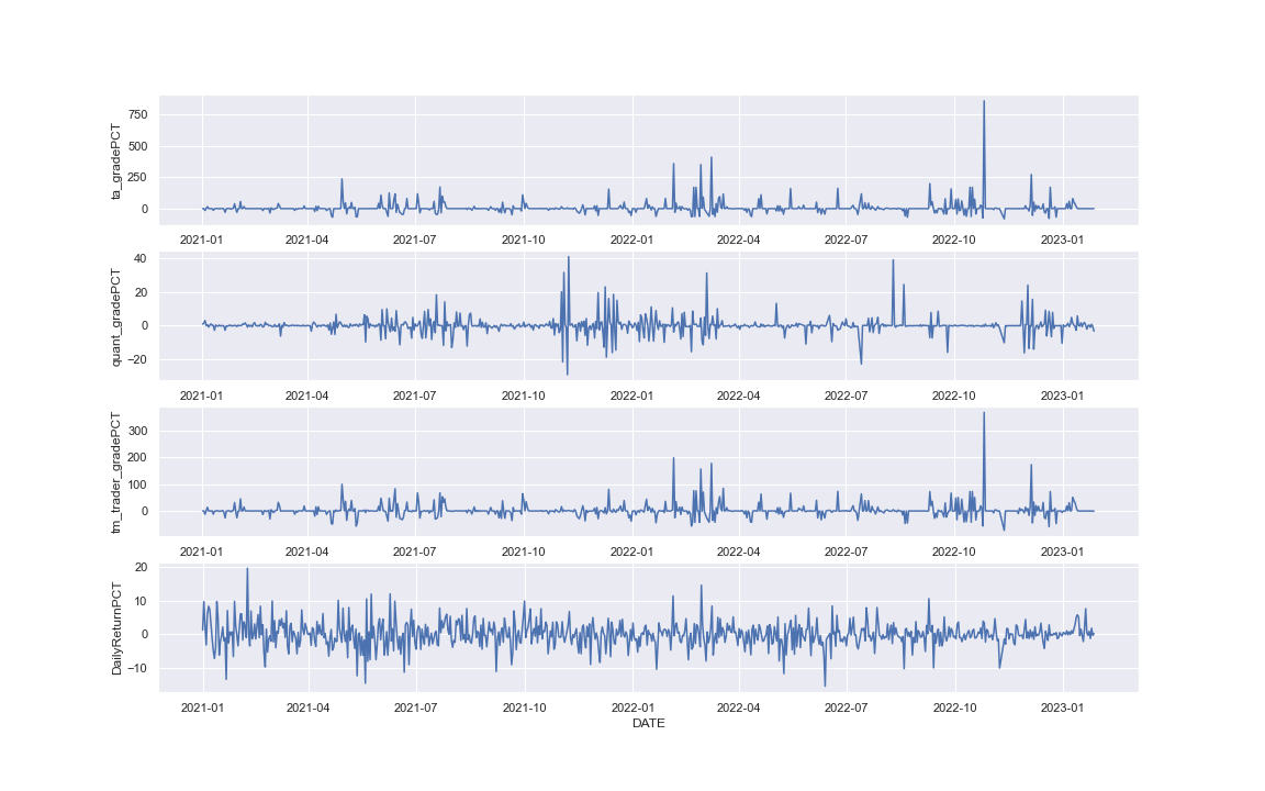
fig = plot_multiTS(data[['TA_GRADE','QUANT_GRADE','TM_TRADER_GRADE','DailyReturnPCT','DATE']], list(range(4)), 'DATE')

From the plots above, we can observe the relationship:

Both the TM_TRADER_GRADE and the TA_GRADE have similar features.
There seems to be a high relationship between the TA_GRADE and the DailyReturnPCT. For example, when we were looking at the high volatility part of the DailyReturnPCT, it is clear that both TM_TRADER_GRADE and TA_GRADE were encountering volatility as well.
QUANT_GRADE contributes little to the DailyReturnPCT.

Let's move further, doing some transformation and statistics.

fig = plot_multiTS(data[['ta_gradePCT','quant_gradePCT','tm_trader_gradePCT','DailyReturnPCT','DATE']], list(range(4)), 'DATE')

Now, let's do simple linear regression to verify this relationship.

fig,axes = plot_regressions(data[['ta_gradePCT','quant_gradePCT','tm_trader_gradePCT']], data['DailyReturnPCT'], plots_in_col = 3)

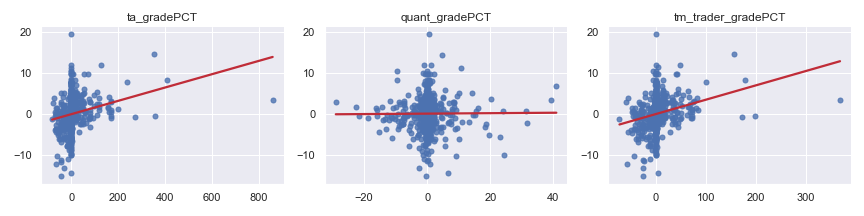
Here we can observe two positive relationships:

ta_gradePCT vs. DailyReturnPCT
tm_trader_gradePCT vs.DailyReturnPCT

Fill null data and save the data for later.

# Handle missing values
data = data.fillna(method='ffill')

data[['DATE','Open','High','Low','Close','Volume','TA_GRADE','QUANT_GRADE','TM_TRADER_GRADE']].sort_values(by = 'DATE').to_csv('../Data/TMdata.csv', index=False)

2.3 Coming up with a Trading Idea

We saw strong and positive relationships for both TA_GRADE, TM_TRADER_GRADE with DailyReturnPCT. Let me give an example to explain the positive relationship and how we can derive a trading idea:

What we have:

DailyReturnPCT = The Close price of the day - the Open price of the day.
Our TM_TRADER_GRADE will be updated at start of the day.
There is a significant positive relationship between the DailyReturnPCT and TM_TRADER_GRADE.

Here is the scenario:

Now it is the Morning of 01/27/2023I received today's TM_TRADER_GRADE of Bitcoin and it shows an upward trend, so I purchasedBitcoin and waited for the day to end.

When it comes to the end of the day of 01/27/2023I sold my Bitcoin position and obtained a 0.1% profit over the day.

What we will do:

Based on the above scenario, let's move it into a more professional description and come up with the following trading logic:

Feature: TM_TRADER_GRADE
Trading pair: BTCUSDT Perpetual
Exchange: Binance US
Buy signal: When the TM_TRADER_GRADE shows an up-trend
Sell signal: When the TM_TRADER_GRADE shows a down-trend
Position: Long, Short
Commission fee: 0.04%
Size: All in
Starting Cash: $100,000
Price slippage: Almost ignorable (24h Volume (USDT) for BTCUSDT Perpetual: $17B)
Frequency: Daily
When entering the market: 00:00:00
When out of the market: 23:59:59

Once we develop this exciting trading strategy, professional backtesting is necessary to verify and measure the design. This is what we will cover in Step 3.